Solute Transport - General

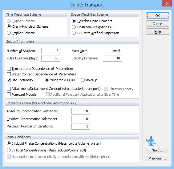
Basic information needed for defining solute transport problem are entered in the Solute Transport dialog window. In this window users specify the Space and Time Weighting Schemes, the Iteration Criteria (for nonlinear problems), and additional Solute Information such as mass units, pulse duration (if applicable), and number of solutes.

a) Time Weighting Scheme

The Time Weighting Scheme defines the temporal weighing coefficient, ε, used in the numerical solution of the transport equation. The temporal weighting coefficient is equal to 0.0 for an explicit scheme, 0.5 for a Crank-Nicholson time-centered implicit scheme, and 1.0 for a fully implicit scheme. The structure of the final set of linear equations [G] {c} = {g}, obtained after the spatial and temporal discretization of the governing advection-dispersion equation, depends upon the value of the temporal weighing factor, ε. The explicit (ε=0) and fully implicit (ε=1) schemes require that the global matrix [G] and the vector {g} be evaluated at only one time level (the previous or current time level). The other two schemes require evaluation at both time levels. Also, the Crank-Nicholson and implicit schemes lead to an asymmetric banded matrix [G]. By contrast, the explicit scheme (ε=0) leads to a diagonal matrix [G] which is much easier to solve (but generally requires much smaller time steps).

The Crank-Nicholson centered scheme is recommended in view of solution precision. The fully implicit scheme also leads to numerical dispersion, but is better in avoiding numerical instabilities. The explicit scheme is most prone to numerical instabilities with undesired oscillations (and is currently disabled).

b) Space Weighting Scheme

HYDRUS provides three options for the Space Weighting Scheme, i.e., the regular Galerkin Finite Elements formulation, the Upstream Weighting Finite Elements formulation, and the Galerkin Finite Elements formulation with Artificial Dispersion.

While the Galerkin Finite Elements formulation is recommended in view of solution precision, Upstream Weighting is provided as an option in HYDRUS to minimize some of the problems with numerical oscillations when relatively steep concentration fronts are being simulated. For this purpose the second (flux) term of advective-dispersive equation is not weighted by regular linear basis functions, but instead using nonlinear functions [Yeh and Tripathi, 1990]. The weighing functions ensure that relatively more weight is placed on flow velocities of nodes located at the upstream side of an element.

Additional Artificial Dispersion may be added also to stabilize the numerical solution and to limit or avoid undesired oscillations in the Galerkin finite element results. Artificial dispersion is added such that a Stability Criterion involving Pe.Cr (the product of the Peclet number and the Curant number) [Perrochet and Berod, 1993] is satisfied. The recommended value for Pe.Cr is 2.0.

c) Solute Information

Number of Solutes        Number of solutes to be simulated simultaneously or involved in a decay chain reaction.

Pulse Duration        Time duration of the concentration pulse. Concentrations (flux or resident) along all boundaries, for which no time-variable boundary conditions are specified, are then set equal to zero for times larger than the "Pulse Duration". When the Fumigant option is active, this variable is used instead to define Time of Tarp Removal.

Mass Units        Units to be printed to the output files or displayed in various graphs. Mass units have no effect on the calculations. Concentration units in general should be given in [ML-3], where M is Mass Units specified in the Solute Transport dialog window (Fig. ) and L is Length Units specified in the Domain Type and Units dialog window (Fig. ). However, since the concentration variable appears in each term of the governing solute transport equations (Eq. 3.1 and 3.2 of the Technical Manual), it is possible to use different length units than those used to define geometry and fluxes (e.g., geometry may be specified in meters while concentrations are given in mg/cm3). In such case the solute fluxes (cq) will then be in units of MLc-3LgT-1 where Lc is the length unit (e.g. cm) used to define concentrations and Lg the length unit defining geometry and fluxes (e.g., m). Similarly the solute mass (cqV) obtained by integrating solute over the transport domain will be in units of MLc-3Lg2. Similar adjustments of units need to be done for other variables that involve both concentration and length units.

Stability Criterion        Product of the dimensionless Peclet and Curant numbers (Pe.Cr). This criterion is used either to add artificial dispersion in the Galerkin Finite Elements with Artificial Dispersion scheme or to limit the time step (leading to lower Courant numbers for a given Peclet number) for the Galerkin Finite Elements scheme.

Use Tortuosity Factor        Check this box when molecular diffusion coefficients in the water and gas phases are to be multiplied by a tortuosity factor according to the formulation of either Millington and Quirk [1961] or Moldrup et al. [1997, 2000].

Temperature Dependence        Check this box if the solute transport and reaction parameters are assumed to be temperature dependent.

Water Content Dependence        Check this box if the solute reaction parameters are assumed to be water content dependent [Walker, 1974].

Attachment/Detachment        Check this box if the solute is assumed to be subject to attachment/detachment to/from the solid phase. This process is often used in simulations of the transport of viruses, colloids, or bacteria.

Filtration Theory        Check this box if the attachment coefficient is to be calculated from filtration theory.

Fumigant Module        Additional options related to fumigant transport (e.g., tarp removal, temperature dependent tarp properties, additional injection of fumigants) can be used with this module.

d) Iteration Criteria

The advection-dispersion solute transport equation becomes nonlinear when nonlinear adsorption is considered. Similarly as for the Richards equation, an iterative process must then be used to obtain solutions of the global matrix equation at each new time step. During each iteration a system of linearized algebraic equations is derived and solved using either Gaussian elimination or the conjugate gradient method. After inversion, the coefficients are re‑evaluated using the initial solution, and the new equations are again solved. This iterative process continues until a satisfactory degree of convergence is obtained, i.e., until at all nodes the absolute change in concentration between two successive iterations becomes less than some concentration tolerance (defined in HYDRUS as the sum of an Absolute Concentration Tolerance and the product of the concentration and a Relative Concentration Tolerance (the recommended and default value is 0.001)). The Maximum Number of Iterations allowed during a certain time step needs to be specified (recommended value is 10). When the Maximum Number of Iterations is reached then the numerical solution is either (a) terminated for problems involving transient water flow or (b) restarted with a reduced time step for steady-state flow problems.

e) Initial Conditions

Initial Conditions can be specified either using liquid phase concentrations in units of mass of solute [Mc] per volume of water [McLw-3] or using total concentrations in units of mass of solute per volume of soil [McLs-3]. In the latter case the liquid phase concentration is calculated from the total concentration depending on the distribution coefficients (e.g., Kd, or Henry’s constant) between different phases.

Rather then specifying directly the initial values of the nonequilibrium phase concentrations (e.g., concentrations in the immobile water for the dual-porosity models or concentrations kinetically sorbed to the solid phase for the two-site sorption models, or for concentrations associated with the solid phase for the attachment/detachment models), users can specify that the nonequilibrium phase concentrations are initially at equilibrium with the equilibrium phase concentrations. Initial conditions need to be then specified only for the liquid phase concentrations, and the nonequilibrium phase concentrations are calculated by HYDRUS.

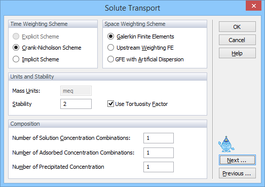
The UNSATCHEM Module

When the UNSATCHEM module is used, basic information needed for defining solute transport problem are entered in the Solute Transport dialog window (instead of the dialog window given above, which is used for the standard solute transport module). In this window users specify again the Space and Time Weighting Schemes, and additional Solute Information such as mass units. Note that all concentrations in the UNSATCHEM module are either in meq/L (in the liquid phase) or meq/kg (in the solid phase) (meq=mmolc). The pulse duration is not used in UNSATCHEM and the number of solutes is fixed to 8 (i.e., the number of considered major ions: Ca2+, Mg2+, Na+, K+, Alkalinity, SO42-, Cl-, and an independent tracer). The number of solution, adsorbed, and precipitated concentration combinations is specified when simulating the transport of major ions in the UNSATCHEM module. This value represents the maximum number of (solution, adsorbed, and precipitated) concentration combinations, which can be used to specify the initial and boundary conditions.

Since there is currently no technical manual describing the two-dimensional version of the UNSATCHEM module, users are referred to the HYDRUS-1D manual [Šimůnek et al., 2008], which provides  all relevant information about this module.