Objective function and statistics

The objective function Φ to be minimized during the parameter estimation process may be defined as [Šimůnek et al., 1998]:

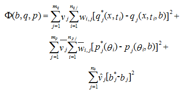
where the first term on the right-hand side represents deviations between the measured and calculated space-time variables (e.g., observed pressure heads, water contents, and/or concentrations at different locations and/or time in the flow domain, or the actual or cumulative flux versus time across a boundary of specified type). In this term, mq is the number of different sets of measurements, nqj is the number of measurements in a particular measurement set, qj*(x,ti) represents specific measurements at time ti for the jth measurement set at location x(r,z), qj(x,ti ,b) are the corresponding model predictions for the vector of optimized parameters b (e.g., θr , θs , α, n, Ks, Dl, kg,k, ...), and vj and wi,j are weights associated with a particular measurement set or point, respectively. The second term of (7.1) represents differences between independently measured and predicted soil hydraulic properties (e.g., retention, θ(h) and/or hydraulic conductivity, K(θ) or K(h) data), while the terms mp, npj, pj*(θi), pj(θi ,b), j and have similar meanings as for the first term but now for the soil hydraulic properties. The last term of (7.2) represents a penalty function for deviations between prior knowledge of the soil hydraulic parameters, bj*, and their final estimates, bj, with nb being the number of parameters with prior knowledge and representing pre-assigned weights. Estimates, which make use of prior information (such as those used in the third term of Φ) are known as Bayesian estimates. We note that the covariance (weighting) matrices, which provide information about the measurement accuracy, as well as any possible correlation between measurement errors and/or parameters, are assumed to be diagonal in this study.

The weighting coefficients vj , which minimize differences in weighting between different data types because of different absolute values and numbers of data involved, are given by [Clausnitzer and Hopmans, 1995]:

which causes the objective function to become the average weighted squared deviation normalized by the measurement variances σj2.

Minimization of the objective function Φ is accomplished by using the Levenberg-Marquardt nonlinear minimization method (a weighted least-squares approach based on Marquardt's maximum neighborhood method) [Marquardt, 1963]. This method combines the Newton and steepest descend methods, and generates confidence intervals for the optimized parameters. The method was found to be very effective and has become a standard in nonlinear least-squares fitting among soil scientists and hydrologists [van Genuchten, 1981; Kool et al., 1985, 1987].

As part of the inverse solution, HYDRUS produces a correlation matrix, which specifies the degree of correlation between the fitted coefficients. The correlation matrix quantifies changes in model predictions caused by small changes in the final estimate of a particular parameter, relative to similar changes as a result of changes in the other parameters. The correlation matrix reflects the nonorthogonality between two parameter values. A value of ±1 suggests a perfect linear correlation whereas 0 indicates no correlation at all. The correlation matrix may be used to select which parameters, if any, are best kept constant in the parameter estimation process because of high correlation.

An important measure of the goodness of fit is the r2 value for regression of the observed, y^i, versus fitted, yi(b), values:

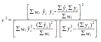
The r2 value is a measure of the relative magnitude of the total sum of squares associated with the fitted equation; a value of 1 indicates a perfect correlation between the fitted and observed values.

HYDRUS provides additional statistical information about the fitted parameters such as the mean, standard error, T-value, and the lower and upper confidence limits (given in output file FIT.OUT). The standard error, s(bj), is estimated from knowledge of the objective function, the number of observations, the number of unknown parameters to be fitted, and an inverse matrix [Daniel and Wood, 1971]. The T-value is obtained from the mean and standard error using the equation

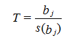
The values for T and s(bj) provide absolute and relative measures of the deviations around the mean. HYDRUS also specifies the upper and lower bounds of the 95% confidence level around each fitted parameter bj. It is desirable that the real value of the target parameter always be located in a narrow interval around the estimated mean as obtained with the optimization program. Large confidence limits indicate that the results are not very sensitive to the value of a particular parameter.

Finally, because of possible problems related to convergence and parameter uniqueness, we recommend to routinely rerun the program with different initial parameter estimates to verify that the program indeed converges to the same global minimum in the objective function. This is especially important for field data sets, which often exhibit considerable scatter in the measurements, or may cover only a narrow range of soil water contents, pressure heads, and/or concentrations. Whereas HYDRUS will not accept initial estimates that are out of range, it is ultimately the user's responsibility to select meaningful initial estimates. Parameter optimization is implemented only for two-dimensional problems.