1. Temporal Discretization
Four different time discretizations are introduced in HYDRUS:
Discretizations 2, 3, and 4 are mutually independent; they generally involve variable time steps as described in the input data file. Discretization 1 starts with a prescribed initial time increment, Δt. This time increment is automatically adjusted at each time level according to the following rules:
a. Discretization 1 must coincide with time values resulting from time discretizations 2, 3, and 4.
b. Time increments cannot become less than a preselected minimum time step, Δtmin, nor exceed a maximum time step, Δtmax (i.e., Δtmin ≤ Δt ≤ Δtmax).
c. If, during a particular time step, the number of iterations necessary to reach convergence is ≤3 (Itmin), the time increment for the next time step is increased by multiplying Δt with a predetermined constant k1>1 (usually between 1.1 and 1.5). If the number of iterations is ≥7 (Itmax), Δt for the next time level is multiplied by a constant k2<1 (usually between 0.3 and 0.9).
d. If, during a particular time step, the number of iterations at any time level becomes greater than a prescribed maximum (usually between 10 and 50), the iterative process for that time level is terminated. The time step is subsequently reset to Δt/3, and the iterative process restarted.
We note that the selection of optimal time steps, Δt, during execution is also influenced by the adopted solution scheme for solute transport.
Parameter |
Recommended Value |
Comment |
Δtinit |
1 s (15 minutes) |
Initial time step, Δt [T]. The recommended value for the initial time step depends on the type of simulation and boundary conditions used. When simulating a process that starts with a large initial pressure head or concentration gradient at the boundary (e.g., ponded infiltration or a sudden change of boundary concentration), use a small value of the initial time step (e.g., 1 s). When simulating a long term process with variable boundary conditions (e.g., seasonal or multiyear simulation), start with a larger time step (e.g., 15 min). This is because this initial time step is used whenever time variable boundary conditions significantly change (e.g., the water flux changes by 25% or more). If needed (if there is no convergence for Δtinit), the program will still use a smaller time step than Δtinit, but starting with larger Δtinit leads to more efficient calculations. In general smaller initial time steps must be used for soil with more nonlinear soil hydraulic properties (e.g., course textured soils) and larger initial time steps can be used for soil with less nonlinear soil hydraulic properties (e.g., loam). |
Δtmin |
1 s |
Minimum permitted value of the time step, Δtmin [T]. The minimum time step must be smaller than a) the initial time step, b) interval between print times, and c) interval between time-variable boundary condition records. Always specify a small minimum allowed time step, on the order of 1 s. This value may never be used, but it provides the code with flexibility when it may be needed, e.g., when there is a sudden change in boundary fluxes and HYDRUS may not converge with larger time steps. |
Δtmax |
Large |
Maximum permitted value of the time step, Δtmax [T]. This is relatively unimportant parameter and a large value may be specified. Since HYDRUS automatically selects its optimal time step, there is usually no need to constraint that. The only time when there is a need to constrain the time step is likely for cases when HYDRUS is asked to generate internally intra-daily variations in temperature, or in evaporation and transpiration fluxes. Then there is a need to have time step smaller (e.g., 1 h) so that these daily variations can be properly modeled. |
Itcrit |
10 |
Maximum number of iterations allowed during any time step while solving the nonlinear Richards equation using a modified Picard method. The recommended and default value is 10. It is usually not helpful to use a larger value than 10. If HYDRUS does not converge in 10 iterations, then there is a relatively small probability that it will do so during more iteration. Even if it does, it is much more efficient to reduce the time step and attempt to find the solution with a smaller time step, which is done automatically by the program when Itcrit is reached. |
Itmin |
3 |
If the number of required iterations at a particular time step is less than or equal to Itmin, then Δt for the next time step is multiplied by a dimensionless number k1 ≥ 1.0. An optimal value in most cases is 3. |
Itmax |
7 |
If the number of required iterations at a particular time step is greater than or equal to Itmax, then Δt for the next time step is multiplied by k2≤ 1.0 (e.g. 0.33). An optimal value in most cases is 7. |
k1 |
1.3 |
Optimal value in most cases. Only when there is a saturated zone in the profile, e.g., a perched water layer, the numerical solution may be more stable with smaller k1 (e.g., 1.1). |
k2 |
0.7 |
Optimal value in most cases. |
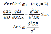
Additionally, the time step is also constrained by stability requirements of the numerical solution of the convection-dispersion solute transport equation:
In HYDRUS, it is possible to vary some variables versus time internally. For example, HYDRUS can generate daily or annual changes in temperature using a sine wave with a prescribed mean temperature and a temperature amplitude. Similarly, HYDRUS can also generate variations of transpiration during the day (see the technical manual). In such case, when time changes of selected variables are generated internally by HYDRUS, it is up to users to limit the maximum time step so that effects of these changes can be properly modeled. For these internally generated time-variable changes (e.g., in temperatures and/or ET), it is recommended to limit the maximum time step to about 1/20 of one time period (e.g., the time step of 0.05 d for a daily cycle).
2. Spatial Discretization
The finite element mesh is constructed by dividing the flow region for two-dimensional problems into quadrilateral and/or triangular elements or for three-dimensional problems into tetrahedral, hexahedral and/or triangular prismatic elements whose shapes are defined by the coordinates of the nodes that form the element corners. The program automatically subdivides the quadrilaterals into triangles (or hexahedrals and triangular prisms into tetrahedrals), which are then treated as subelements.
Common Rules
In general, the finer the FE-mesh size is, the more precise the results will be. On the other hand, the number of calculation steps increases, as additional equations must be solved for every further FE node. This affects the computing time considerably. A mesh size that is too fine slows down the calculation without improving the quality of the analysis significantly. On the other hand, a coarse mesh may not capture the boundary conditions in a satisfying way and the numerical solution may not converge.
Finite element dimensions must be adjusted to a particular problem. They should be made relatively small at locations where large hydraulic gradients are expected. Such a region is usually located close to the soil surface where highly variable meteorological factors can cause rapid changes in the soil water content and corresponding pressure heads. Similarly, regions with sharp gradients can be located in the vicinity of the internal sources or sinks. Hence, we recommend normally using relatively small elements at and near the soil surface. The size of elements can gradually increase with depth to reflect the generally much slower changes in pressure heads at deeper depths. We also recommend using elements having approximately equal sizes to decrease numerical errors. The ratio of the sizes of two neighboring elements is not recommended to exceed about 1.5.
The required size of finite elements close to the soil surface depends very much on how boundary conditions are specified. When boundary conditions are specified for daily, or shorter, time intervals, usually resulting in short-duration fluxes of a large magnitude, spatial discretization needs to be finer (on the order of cm) than when boundary conditions are specified for longer time intervals (e.g., weekly or monthly).
The element dimensions should also depend upon the soil hydraulic properties. For example, coarse-textured soils having relatively high n- and α-values generally require a finer discretization than fine-textured soils. That is because their soil hydraulic functions are more nonlinear and thus the numerical solution may be less stable. To demonstrate this issue, we have carried out simulations of ponded infiltrations into sand and clay soil profiles (see Figure below). Notice that the pressure head front for a sandy profile is very sharp and the entire front is only about 5 cm thick. To be able to describe this front using our numerical model, we need several FE nodes at the front, implying that our spatial discretization must be on the order of 1 cm or less. On the other hand, the pressure head (and correspondingly water content) front for a clay profile is relatively smooth and consequently our spatial discretization can be much coarser.
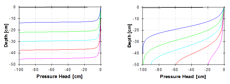
Pressure head profiles for ponded infiltration into sand and clay soil profiles.
In higher dimensions, it is often recommended that in order to obtain smooth solutions, FE elements should have approximately all sides equal. This recommendation is not valid for most applications involving fluxes in the vadose zone. Since in the vadose zone vertical fluxes usually dominate over horizontal fluxes, the spatial discretization must be much finer in the vertical direction than in the horizontal direction. In general, the spatial discretization should reflect the expected gradients in the transport domain; it should be fine in the direction of large gradients and can be coarser in the direction of small gradients.
HYDRUS offers several parameters and tools to adjust the spatial discretization to expected flow and transport conditions. The four most important parameters and tools are the Targeted FE Size, the Smoothing Factor, Mesh Stretching, and the FE-Mesh Refinement. The first three parameters can be specified in the FE Mesh Parameters dialog window, which can be displayed by clicking on the menu command “Edit->FE-Mesh->FE-Mesh Parameters” or the FE-Mesh Parameters command ( ) at the Tools Sidebar when the FE-Mesh View is displayed.
HYDRUS uses two different FE-Mesh generation modules. It uses the MeshGen module to generate FE meshes for two-dimensional domains and for the Base Surface of three-dimensional layered domains. It then uses the Genex/T3D module to generate FE meshes for three-dimensional general domains (note that three-dimensional general domains are available only in the 3D-Professional Level of HYDRUS). These are relatively different approaches to generating FE meshes and thus the use of the above discussed parameters and tools is sometimes also different. In the text below we will attempt to emphasize these differences.
Targeted FE Size
The Targeted FE Size defines the global FE mesh size, i.e., the size of finite elements that the FE-Mesh generator will try to reach throughout the transport domain. FE-Mesh can be made finer or coarser in different parts of the transport domain by defining FE-Mesh Refinements (see discussion below) for these parts of the domain.
Note that the Targeted FE Size that is suggested by HYDRUS (when the check box Automatic is on) is related only to the size of the transport domain, and is a certain fraction (e.g., 1/60) of the diameter of the transport domain. The purpose of this number is to suggest such size of finite elements, so that the number of elements is reasonable. The Automatic Targeted FE Size is not adjusted to any other factors involved in a particular project, such as nonlinearity of soil hydraulic properties, how the boundary conditions are defined, heterogeneity of the soil profile, and so on. Users need to adjust the Targeted FE Size for their particular problems themselves and then adjust the FE-mesh where needed using FE-Mesh Refinements as needed.
Note that the Targeted FE Size is used by GENEX in all three dimensions and by MeshGen in two dimensions (for the Base Surface of Layered Three-Dimensional domains). Distances between layers in Layered Three-Dimensional domains is defined differently (see below).
Smoothing Factor
The Smoothing Factor (see Figure below) is the ratio of the maximum and minimum height of a finite element triangle. The Smoothing Factor is used only in for FE-meshes generated using MeshGen, i.e., for 2D and 3D-Layered domains, but not for FE-meshes generated using Genex, i.e., for 3D-General domains. For a triangle with equal sizes this factor is equal to 1 (which is theoretically not achievable for finite element meshes). The Smoothing Factor can be decreased to a value of about 1.1 when a highly smooth finite element mesh is required and, vice-versa, can be increased when a course mesh can be tolerated. The Smoothing Factor significantly affects the final number of elements, with the number of elements decreasing dramatically for larger values of the smoothing factor (e.g., 3). We recommend keeping the Smoothing Factor at its default value (i.e., 1.3) for relatively small transport domains (e.g., simulations of irrigation details), and increase its value to about 2-3 for larger transport domains (e.g., soil transects, field scale simulations) (see Figure below).
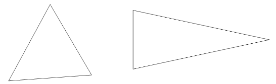
Triangles with a smoothing factor equal to 1 (left) and 3 (right).
Stretching
Stretching of the finite element mesh (i.e., the degree of mesh anisotropy in a certain direction) is defined using the Stretching Factor and the Stretching Direction (see Figure below). The finite elements are made larger in the particular Stretching Direction and the Stretching Factor is larger than one, and smaller if it is less that one. The result of this transformation is a mesh deformed in the given direction, which can be desirable for problems that, for example, require different spatial steps (mesh sizes) in the X, Y, and Z directions. As discussed above, in the vadose zone vertical fluxes usually dominate over horizontal fluxes, and thus the spatial discretization must be much finer in the vertical direction than in the horizontal direction. If vertical fluxes are expected to be many times larger (e.g., 10-100 times) in the vertical direction than in the horizontal direction, the Stretching Factor can also be very large (e.g., 10-100).
Example of mesh stretching using a stretching factor of 3 in the x-direction.
FE-Mesh Refinement
If no FE-Mesh Refinement have been defined, the FE mesh is generated with the preset Targeted FE Size.
The mesh configuration can be affected by FE-Mesh Refinement that are set for selected parts of the computational domain. Use this option to refine the mesh where needed, such as at parts of the computational domains where large pressure head and/or concentration gradients are expected. Large pressure head and/or concentration gradients usually occur close to the soil surface (due to variable atmospheric fluxes), close to internal sinks/sources (drains, drippers, wells), or close to interfaces between different soil layers with significantly different soil hydraulic properties.
Using FE-Mesh Refinements one may try to find an appropriate compromise between results accuracy and computational time. Basically, there are four types of FE-Mesh Refinements:
• Refinement around a node
• Refinement on a line
• Refinement on a surface
• Refinement on a solid (used only with Genex)