Root Growth

The HYDRUS models now include a relatively comprehensive macroscopic root water and solute uptake module (Šimůnek and Hopmans, 2009) to account for both water and salinity stress effects on water uptake, while also accounting for possible active and passive root solute uptake. Root water and solute uptake furthermore can be treated as being either non-compensated or compensated.

HYDRUS-1D additionally also allows users to externally prescribe a time-variable rooting depth, either using the logistic growth function or in a tabulated form. Such a feature has not been available in HYDRUS (2D/3D), which has been a common complaint of many HYDRUS users. The spatial distribution of roots in the root zone was assumed to remain constant during the simulations and only the intensity of uptake (as a result of time-variable potential transpiration) could be specified at the input. Both models also do not allow the spatial extent of the rooting zone to change actively as a result of environmental stresses.

To overcome these deficiencies, several studies either further modified the HYDRUS models (or their predecessors such as CHAIN-2D or SWMS-3D), or coupled the models with various crop growth or root growth models. For example, Javaux et al. (2008, 2013), developed R-SWMS, a three-dimensional root growth model that couples the model of Somma et al. (1998) (based on SWMS-3D) with the model of Doussan et al. (1998). Zhou et al. (2012) coupled HYDRUS-1D with the WOFOST (Boogaard et al., 1998) crop growth model and used the resulting model to simulate the growth and yield of irrigated wheat and maize (Li et al., 2012, 2014). Han et al. (2015) similarly coupled HYDRUS-1D with a simplified crop growth version used in SWAT to simulate the contribution and impact of groundwater on cotton growth and root zone water balance. Wang et al. (2014) and Wang et al. (2015) coupled the crop growth model EPIC (Williams et al., 1989) with CHAIN-2D and HYDRUS-1D to assess the effects of furrow and sprinkler irrigation, respectively, on crop growth. Finally, Hartmann et al. (2017) implemented into both HYDRUS-1D and HYDRUS (2/3D) the root growth model developed by Jones et al. (1991). Their model assumes that various environmental factors as characterized by growth stress factors, can influence root development under suboptimal conditions. Only the models of Hartmann et al. (2017) are directly available from the HYDRUS website as a non-standard HYDRUS module, i.e., not fully supported by the HYDRUS GUI.

To extend the capabilities of the standard module of HYDRUS (2D/3D), a simple root growth model, with similar capabilities to those in HYDRUS-1D, was implemented into Version 3. The rooting depth, LR, can be either constant (the standard approach) or variable during the simulation. For annual vegetation a growth model is required to simulate the change in rooting depth with time. The time-variable rooting depth values can be either provided in the table on the input, or the program can calculate the time variable rooting depth assuming that the actual root depth is the product of the maximum rooting depth, Lm [L], and the root growth coefficient, fr(t) [-]:

For the root growth coefficient, fr(t), we use the classical Verhulst-Pearl logistic growth function

where L0 is the initial value of the rooting depth at the beginning of the growing season [L], and r the growth rate [T-1]. The growth rate, r, can be calculated either from the assumption that 50% of the rooting depth will be reached after 50% of the growing season has elapsed, or from given data of the root depth at a specified time. The same approach is also used for the horizontal extent of the rooting zone, except that the maximum extent of the rooting zone in the horizontal direction is used instead of the maximum rooting depth.

When variable rooting depth is considered, the spatial distribution of roots must be described using either the Vrugt (Vrugt et al., 2001ab) or Hoffman and van Genuchten (Hoffman and van Genuchten, 1983) functions. The Vrugt two-dimensional root distribution function is implemented in HYDRUS as follows (Vrugt et al., 2001ab):

where Xm and Zm are the maximum rooting lengths in the x- and z- directions [L], respectively; x and z are distances from the origin of the plant (tree) in the x- and z- directions [L], respectively; px [-], pz [-], x* [L], and z* [L] are empirical parameters (x* and z* are Depth of Maximum Intensity or Radius of Maximum Intensity; parameters px and pz are assumed to be zero for x> x*, z> z*, respectively (Vrugt et al., 2001ab)), and b(x,z) denote two- -dimensional spatial distribution of the potential root water uptake [-]. See Vrugt et al. (2001ab) for different configurations of the normalized spatial distribution of potential root water uptake rate.

Alternatively, one can use the following function (Hoffman and van Genuchten, 1983):

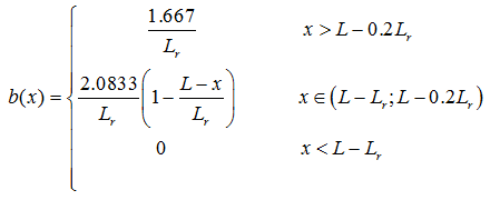
where L is the x-coordinate of the soil surface [L] and Zm is the root depth [L].

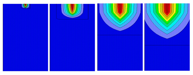
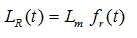
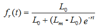
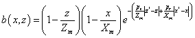
An example of the two-dimensional spatial distribution of the root water uptake is shown below for the following root growth parameters: L0=5 cm, Zm=Lmz=100 cm, Xm=Lmx=75 cm, x*=0, z*=20 cm, px=pz =1.