The Time Variable Boundary Conditions dialog window is shown below.
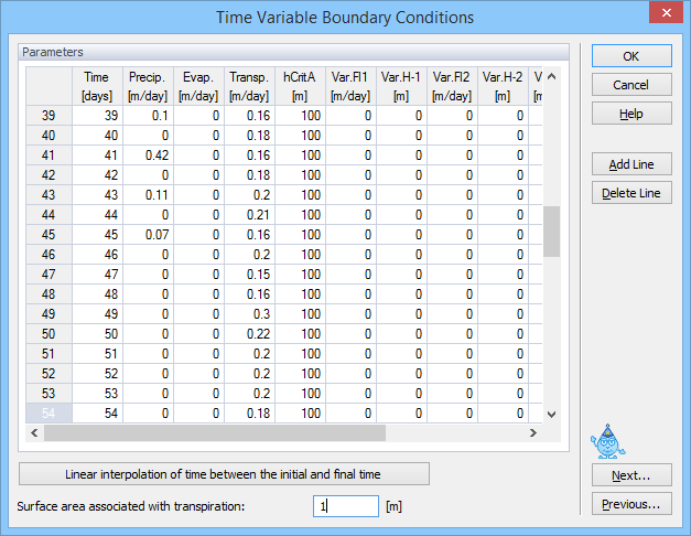
The following variables are specified in the Time Variable Boundary Conditions dialog window:
Time |
Time for which a data record is provided [T]. Boundary condition values are specified for the time interval preceding time given at the same line. Thus, the BC values specified on the first row are for the time interval between the initial time and time specified on the same line. |
Precip |
Precipitation rate [LT-1] (in absolute value) (applied to the atmospheric boundary). |
Evap |
Potential evaporation rate [LT-1] (in absolute value) (applied to the atmospheric boundary). |
Trans |
Potential transpiration rate [LT-1] (in absolute value). |
hCritA |
Absolute value of the minimum allowed pressure head at the soil surface [L] (applied to the atmospheric boundary). hCritA should be selected such so that the corresponding water content is at least 0.005 higher than the residual water content. It should also be lower (when negative) than P3 when the root water uptake is considered. When both limits for root water uptake (P3) and evaporation (hCritA) are reached, hCritA>P3 leads to inflow since it controls the flux across the boundary. |
Var.Fl1 |
Drainage flux [LT-1] across the bottom boundary, or another time-dependent prescribed flux boundary condition (positive when water leaves the flow region); set to zero when no time-dependent flux boundary condition is specified. Same for Var.Fl2, Var.Fl3, or Var.Fl4. The Var.Fl4 value is used for internal time-variable nodal flux sinks or sources (if they exist). When there are time-variable internal nodal flux sinks or sources in the transport domain, time-variable nodal fluxes have to be given in the Var.Fl4 column (in such case, the units are [L2T-1] or [L3T-1] for 2D or 3D applications, respectively). Note that Var.Fl1 values are negative for inflow into and positive for outflow out of the domain. |
Var.H-1 |
Groundwater level [L] (usually negative), or other time-dependent prescribed head boundary condition; set equal to zero when no time-dependent head boundary condition is specified. Same for Var.H-2, Var.H-3, or Var.H-4. The Var. H-4 value is used for internal time-variable nodal pressure head sinks or sources (if they exist). When there are time-variable internal nodal flux sinks or sources in the transport domain, time-variable nodal pressure heads have to be given in the Var.H-4 column. |
TVal1 |
The first time-dependent temperature [K] that can be used for nodes with time variable boundary conditions (atmospheric BC, variable head/flux BC) (is not specified when heat transport or time variable boundary conditions are not considered). |
TVal2 |
The second time-dependent temperature [K] that can be used for nodes with time variable boundary conditions (is not specified when heat transport or time variable boundary conditions are not considered). |
CVal1 |
The first time-dependent solute concentration [ML-3] that can be used for nodes with prescribed time variable boundary conditions (atmospheric BC, variable head/flux BC) (not specified when solute transport is not considered). This column should be used preferably only for the atmospheric boundary, because the concentration value is adjusted based on values of precipitation and evaporation as follows: cVal1=Precip/(Precip-Evap)*cVal1. The cVal1 is adjusted to be zero when Evap > Precip. Similar adjustments are not done for cVal2, and other concentration values. When Unsatchem or HP1 modules are used, cValue1 is the number of the solution composition to be used at the boundary. |
CVal2 |
The second time-dependent solute concentration [ML-3] that can be used for nodes with prescribed time variable boundary conditions (atmospheric BC, variable head/flux BC) (not specified when solute transport is not considered). |
CVal3 |
The third time-dependent solute concentration [ML-3] that can be used for nodes with prescribed time variable boundary conditions (atmospheric BC, variable head/flux BC) (not specified when solute transport is not considered). When the active solute uptake and only one solute is considered, then this column is used to specify the Potential Solute Uptake Rate [ML-2T-1]). |
The last three entries are entered for each solute.
The table can be edited by manually adding or deleting lines. The table has a capacity for about 32,000 records (depends on the number of columns). When a longer time record is to be simulated, then one needs to directly edit the Atmosph.in input file in the working directory using any standard software, such as MS Excel. The manually modified Atmosph.in file then needs to be imported back into the HYDRUS project_name.h32d file using the command File->Import and Export->Import Input Data from *.In Files. Data for the Time Variable Boundary Conditions can be prepared in any spreadsheet software and then copied into the table using Windows paste hot keys (i.e., Ctrl+V).
The total number of atmospheric data records is given in the Main Time Information dialog window.
Surface Area Associated with Transpiration: The total transpiration flux from a simulated transport domain is equal to the potential transpiration Tp (L/T) multiplied by the Surface boundary Area (length in 2D) Associated with Transpiration (see Figure 2.2. of the Technical Manual). It is usually the entire soil surface (usually the boundary area/length with an atmospheric boundary condition). By dissociating this value (i.e., the surface area associated with transpiration) from the surface boundary area/length of the transport domain, we provide HYDRUS users with more flexibility how to specify transpiration (e.g., for sparsely vegetated soil surface, or for row crops or trees). In any case, the definition of the Surface Area Associated with Transpiration depends on how the potential transpiration, Tp, is calculated, which is usually done for the entire soil surface.
Potential Evapotranspiration:
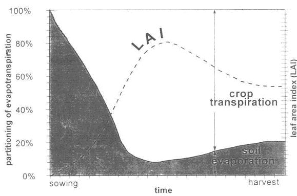
HYDRUS requires users to enter values of potential transpiration and potential evaporation for the atmospheric boundary conditions. HYDRUS then calculates the actual values of transpiration and evaporation based on the availability of water in the soil profile. A common scenario is that users usually know the value of the potential evapotranpiration rate (as calculated for example with the Penman-Monteith combination equation) and not directly its structural parts. Since HYDRUS does not have a crop growth module (does not calculate crop growth, various growth stages, leaf area index, etc) and focuses only on water and solute transport in the soil profile, it can not separate itself the potential evapotranspiration rate into potential evaporation and potential transpiration rates. This division is different for each crop and is relatively complex. FAO and several other publications suggest using a "Crop coefficient" to implement this division (into potential evaporation and potential transpiration). One can also use the Leaf Area Index (LAI) or Surface Fraction covered by plants for this division.
Example of the partitioning of potential ET into potential Evaporation and potential Transpiration based on LAI.
hCritA is the minimum allowed pressure head at the soil surface. This value can be activated only by evaporation. As long as the pressure head at the soil surface is higher then hCritA, the actual evaporation rate is equal to the potential evaporation rate. Once the hCritA value is reached, the actual evaporation rate is decreased from the potential value since the soil is then too dry to deliver the potential rate. The hCritA value is not used for any other calculations. The hCritA value is usually specified in the range of -150 m to -1000 m (it may need to be lower for coarse-textured soils - see the discussion below).
hCritA should be selected such so that the corresponding water content is at least 0.005 higher than the residual water content. This may be important especially for coarse-textured soils (sands), which have a very steep retention curve. For coarse-textured soils, small changes in water contents in the dry range lead to large changes in the pressure heads, which can make the numerical solution unstable. It may thus be needed to use a relatively small value of hCritA.
hCritA should also be lower (when negative) than P3 when the root water uptake is considered. When both limits for root water uptake (P3) and evaporation (hCritA) are reached, hCritA>P3 leads to inflow since it controls the flux across the boundary.
hCritA should be selected such so that the corresponding water content is at least 0.005 higher than the residual water content. It should also be lower (when negative) than P3 when the root water uptake is considered. When both limits for root water uptake (P3) and evaporation (hCritA) are reached, hCritA>P3 leads to inflow since it controls the flux across the boundary.
hCritA can be obtained from the following equation:
Hr=exp(hMg/RT)
where Hr is the relative humidity, g is the gravitational acceleration [LT-2] (=9.81 m s-2), M is the molecular weight of water [M mol-1] (=0.018015 kg mol-1), R is the universal gas constant [J mol-1K-1, ML2T-2mol-1K-1] (=8.314 J mol-1K-1), T is the absolute temperature [K], and h is the pressure head [L].