Reservoir Boundary Condition

Version 3 of the two-dimensional module of HYDRUS (2D/3D) offers a new system-dependent boundary condition, further referred to as the Reservoir Boundary Condition. This option allows users to consider a reservoir that is external to the HYDRUS transport domain, while water can be added (injected) to or removed (pumped) from the reservoir. Flow into or out of the reservoir through its interface with the subsurface transport domain depends on the prevailing conditions in the transport domain (e.g., the position of the groundwater table) and external fluxes. Since mass balances of water and solute in the external reservoir are constantly being updated (based on all incoming and outgoing fluxes), the boundary conditions along the transport domain are dynamically adjusted depending upon the water level in the reservoir.

The Reservoir BC is implemented in HYDRUS (2D/3D) for three different geometries: a well, a furrow, and a wetland. While the furrow BC is implemented only for two-dimensional transport domains, the well and wetland BCs are implemented for both two-dimensional planar and axisymmetric transport domains.

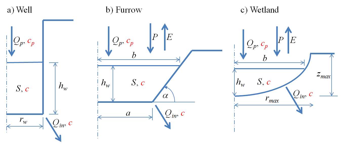
Three different types of the reservoir boundary condition: a well, a furrow, and a wetland. In the figure hw is the water level in the reservoir [L], S is the volume of water in the reservoir ([L2] or [L3] for two-dimensional and axisymmetric systems, respectively), Qp is the pumping rate (positive for removal of water, negative for adding water) ([L2T-1] or [L3T-1] for two-dimensional and axisymmetric systems, respectively), c is the solute concentration in reservoir water [ML-3], cp is the solute concentration in injected water [ML-3], P and E refer to the precipitation and evaporation rates [LT-1], rw is the radius of the well [L], a is the a half-width of the furrow [L], α is the slope of the furrow side [-], rmax is the maximum width (radius) of the wetland [L], zmax is the maximum depth of the wetland [L], and b represents the width of the water table ([L] or [L2] for two-dimensional and axisymmetric systems, respectively).

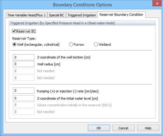
The parameters for the Reservoir Boundary Condition are specified using the Reservoir Boundary Condition Tab of the Boundary Conditions Options dialog window. Users have to first check the Reservoir BC check box and select the Reservoir Type, which can be either Well (rectangular, cylindrical), Furrow, or Wetland . Users have then to provide information about the reservoir geometry (i.e., the z-coordinate of the well (furrow, wetland) bottom, Well (Wetland) Radius or Half Width of the Furrow Bottom, initial position of the water table in the reservoir (Z-coordinate of the initial water level), and Pumping or Injection Rate. When solute transport is considered, then the Solute concentration initially in the reservoir water needs to be specified as well. The Pumping or Injection Rate specified in this window is considered to be constant in time. When time-variable pumping or injection of water from/into reservoir is to be simulated, this rate needs to be provided using the "Var.Fl.-1" column in the Time Variable Boundary Conditions dialog window. Note that this rate is in units of [L2T-1] or  [L3T-1] for two-dimensional or axisymmetrical applications. An output file WELL.OUT is created when the reservoir boundary condition is used containing information about fluxes into and from a reservoir (see Table 11.10 of the Technical Manual).

Back to Boundary Condition Options.

See also the "How to Edit Boundary Conditions" topic.