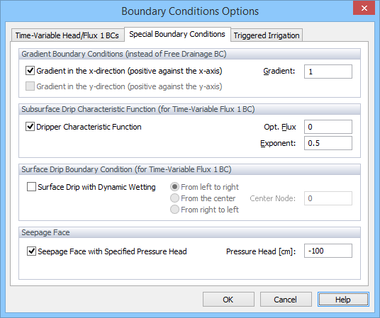
The following Special Boundary Conditions can be selected from the second tab of the Boundary Condition Options dialog window:
Gradient Type Boundary Condition
Version 1 of HYDRUS implements the Gradient Type Boundary Condition only as the Free Drainage boundary condition, or the unit gradient boundary condition. However, in many situations one needs a non-unit gradient BC. For example, it is difficult to select appropriate boundary conditions for vertical boundaries for flow in a hill slope where the side-gradient is more or less parallel with the direction of the slope. In version 2 of HYDRUS, users can specify a gradient other than one (unit gradient). This option, i.e., non-unit gradient boundary condition, needs to be selected from the Special Boundary Conditions tab of the Boundary Condition Options dialog window. Gradients are positive for flow against a particular axis, i.e., from right to left (in the x-direction) and from back to front (in the y-direction), and should be used only (or mainly) on sides of the transport domain. In 3D, the gradient BC can be specified only in one direction (i.e., either in x- or y-direction).
Subsurface Drip Characteristic Function
Infiltration rate of water from a subsurface cavity (dripper) is affected by many factors, including the pressure in the cavity, its size and geometry, and the hydraulic properties of the surrounding soil [Lazarovitch et al., 2005]. When a predetermined discharge of a subsurface source (e.g., a subsurface emitter) is larger than the soil infiltration capacity, the pressure head in the source outlet increases and becomes positive. The built up pressure may significantly reduce the source discharge rate. A special system-dependent boundary condition for flow from subsurface sources that uses the drip characteristic function was implemented in HYDRUS (see the Technical manual). This function has two variables, i.e., the nominal discharge (Optimal Flux in Fig. above) of the source for the reference inlet pressure hin (usually being 10 m) and the back pressure equal to zero, and an empirical constant (Exponent in Fig. above) that reflects the flow characteristics of the emitter. Normally, c = 0.5 corresponds to a turbulent flow emitter and c = 1 to a laminar one. This option is currently available only for two-dimensional and axisymmetrical geometries.
Implementation: User needs to specify the “Time-Variable Flux 1” boundary condition along the dripper boundary and hin in the “Var.H-1” column of the “Time Variable Boundary Conditions” dialog window. A positive pressure indicates an irrigation period and a negative pressure indicates a non-irrigation period.
Surface Drip Irrigation – Dynamic Evaluation of the Wetted Area
The radius of the wetted area for drip irrigation for transient conditions can be calculated in Hydrus as follows. The irrigation flux Q is applied to the single boundary node that represents the dripper with the Neumann (flux) boundary condition. If the pressure head required to accommodate the specified flux Q is larger than zero, the boundary condition in this particular node is changed into the Dirichlet (head) boundary condition with zero pressure head value and the actual infiltration flux Qa through this node is calculated. The excess flux (Q - Qa) is then applied to the neighboring node, again with the specified Neumann boundary condition. This procedure is iteratively repeated until the entire irrigation flux Q is accounted for and the radius of the wetted area is obtained. Since the infiltration flux into the dry soil is larger for early times, the wetted area continuously increases as irrigation proceeds. This option is currently available only for two-dimensional and axisymmetrical geometries.
Implementation: User needs to specify the “Time-Variable Flux 1” boundary condition at the surface boundary. The length of this boundary needs to be sufficient to accommodate the entire wetting zone. The drip discharge flux, Q, needs to be entered in the “Var.Fl-1” column of the “Time Variable Boundary Conditions” dialog window. User also needs to specify from which node of the Time-Variable Flux 1 boundary irrigation starts. Irrigation can start in the left node of the boundary and then the wetting zone will be spreading to the right (From left to right), it can also starts in the right node of the boundary and then the wetting zone will be spreading to the left (From right to left), or it can start in the arbitrary middle node of the boundary (Center Node) and spread in both direction (From the center).
Seepage Face with a Specified Pressure Head
This type of boundary condition is often applied to laboratory soil columns when the bottom of the soil column is exposed to the atmosphere (gravity drainage of a finite soil column). The condition assumes that the boundary flux will remain zero as long as the pressure head is negative. However, when the lower end of the soil profile becomes saturated, a zero pressure head is imposed at the lower boundary and the outflow calculated accordingly. This type of boundary condition is often used for lysimeters.
User can specify a pressure head value other than zero (Pressure Head) for triggering flux across the seepage face (in several experimental settings, a negative pressure can be applied at the bottom of laboratory columns or lysimeters).
Back to Boundary Condition Options.
See also the "How to Edit Boundary Conditions" topic.