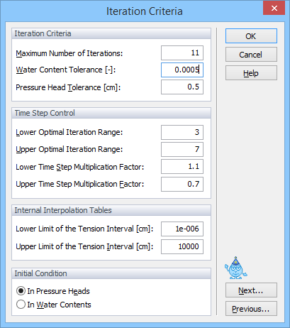
Iteration Criteria

Iteration Criteria

The Iteration Criteria dialog window contains information related to the iterative process that is used to solve the Richards equation. Because of the nonlinear nature of the Richards equation, an iterative process must be used to obtain solutions of the global matrix equation at each new time step. For each iteration a system of linearized algebraic equations is first derived and then solved using either Gaussian elimination or the conjugate gradient method. After solving the matrix equation, the coefficients are re‑evaluated using this solution, and the new equations are again solved. The iterative process continues until a satisfactory degree of convergence is obtained, i.e., until for all nodes in the saturated (unsaturated) region the absolute change in pressure head (water content) between two successive iterations becomes less than some small value determined by the imposed absolute Pressure Head (or Water Content) Tolerance. The first estimate (at zero iteration) of the unknown pressure heads at each time step is obtained by extrapolation from the pressure head values at the previous two time levels.

We do not recommend to change these default values unless you are an experienced user and know exactly what you are doing!

In the Iteration Criteria part of the dialog window, one specifies the maximum number of iterations during one time step, and the water content and pressure head precision tolerances.

Max. Number of Iterations        Maximum number of iterations allowed during any time step while solving the nonlinear Richards equation using a modified Picard method. The recommended and default value is 10. It is usually not helpful to use a larger value than 10. If HYDRUS does not converge in 10 iterations, then there is a relatively small probability that it will do so during more iteration. Even if it does, it is much more efficient to reduce the time step and attempt to find the solution with a smaller time step, which is done automatically by the program when Itcrit is reached.

Water Content Tolerance        Absolute water content tolerance for nodes in the unsaturated part of the flow region [-]. When the water contents between two successive iterations during a particular time step change less than this parameter, the iterative process stops and the numerical solution proceeds to the new time step. Its recommended and default value is 0.001.

Pressure Head Tolerance        Absolute pressure head tolerance for nodes in the saturated part of the flow region [L]. When the pressure heads between two successive iterations during a particular time step change less than this parameter, the iterative process stops and the numerical solution proceeds to the new time step. Its recommended and default value is 1 cm.

Information specified in the Time Step Control part of the dialog window is related to the automatic adjustment of the time step during calculations. Four different time discretizations are introduced in HYDRUS: (1) time discretizations associated with the numerical solution, (2) time discretizations associated with implementation of boundary conditions, (3) time discretizations associated with data points used in the inverse problem, and (4) time discretizations which provide printed output of the simulation results (e.g., nodal values of dependent variables, water and solute mass balance components, and other information about the flow regime).

Discretizations 2, 3, and 4 are mutually independent; they generally involve variable time steps as described in the input data file (Time-Variable Boundary Conditions  and Output Information. Discretization 1 starts with a prescribed initial time increment, Δt. This time increment is automatically adjusted at each time level according to the following rules:

       a.        Discretization 1 must coincide with time values resulting from time discretizations 2, 3, and 4.

       b.        Time increments cannot become less than a preselected minimum time step, Δtmin, nor exceed a maximum time step, Δtmax (i.e., Δtmin ≤ Δt ≤ Δtmax).

       c.        If, during a particular time step, the number of iterations necessary to reach convergence is ≤3, the time increment for the next time step is increased by multiplying Δt with a predetermined constant >1 (usually between 1.1 and 1.5). If the number of iterations is ≥7, Δt for the next time level is multiplied by a constant <1 (usually between 0.3 and 0.9).

       d.        If, during a particular time step, the number of iterations at any time level becomes greater than a prescribed maximum (usually between 10 and 50), the iterative process for that time level is terminated. The time step is subsequently reset to Δt/3, and the iterative process restarted.

We note that the selection of optimal time steps, Δt, during execution is also influenced by the adopted solution scheme for solute transport.

Time Step Control variables.

Internal Interpolation Tables.

At the beginning of a numerical simulation, HYDRUS generates for each soil type in the flow domain a table of water contents, hydraulic conductivities, and specific water capacities from the specified set of hydraulic parameters. Values of the hydraulic properties are then computed during the iterative solution process using linear interpolation between entries in the table. If the pressure head h at some node falls outside the prescribed interval (ha, hb), the hydraulic characteristics at that node are evaluated directly from the hydraulic functions (i.e., without interpolation). The above interpolation technique was found to be much faster computationally than direct evaluation of the hydraulic functions over the entire range of pressure heads. Interpolation using tables can be avoided by setting ha and hb both to zero. Then the soil hydraulic properties are always evaluated directly from the hydraulic functions (i.e., without interpolation). Output graphs of the soil hydraulic properties will be given also for the interval (ha, hb).

Initial Conditions

Finally, in the Initial Conditions part of the dialog window, a user specifies whether the initial conditions for the water flow calculations are to be specified in terms of the pressure head or water content.