The following types of boundary conditions are available for water flow.

Some Boundary Conditions need a single parameter (e.g., Constant Pressure Head or Constant Flux), some need multiple parameters (e.g., Variable Pressure Head, Variable Flux, and Atmospheric BCs need a time-variable sequence of values), and some do not need any parameters (e.g., No Flux BC, Free Drainage, or Seepage Face).

Boundary Conditions

Two types of boundary conditions can be specified on boundaries of the transport domain: system-dependent and system-independent boundary conditions. System-independent boundary conditions are boundary conditions for which the specified boundary value (i.e., pressure head, water content, water flux, or gradient) does not depend on the status of the soil system. System-dependent boundary conditions are boundary conditions for which the actual boundary condition (again either pressure head, water content, water flux, or gradient) depends on the status of the system and is calculated by the model itself.

System-Independent Boundary Conditions

Several system independent boundary conditions may be applied to the transport domain boundaries. When the pressure head at the boundary is known, one can use the Dirichlet boundary condition:

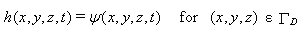
where h0 is a prescribed pressure head [L] at the ΓD Dirichlet boundary segments. This boundary condition is often also referred to as a pressure head boundary condition, or a first-type boundary condition. This boundary condition must be used when simulating ponded infiltration, for describing the hydrostatic pressure at the boundary between the porous material (soil) and standing or flowing water in a furrow, lake or river, to specify the water level in a well, or the define the position of the groundwater table. The water flux across a Dirichlet boundary is not known a priori, but must be calculated from the mathematical solution (either analytical or numerical) of the governing flow problem.

When the water flux across the boundary is known, one can use the Neumann boundary condition:

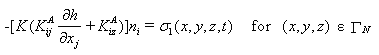
where q0 is a prescribed water flux [LT-1] at the ΓN Neumann boundary segments, and ni are the components of the outward unit vector normal to boundary ΓN . This boundary condition is often also referred to as a flux boundary condition, or a second-type boundary condition. Neumann boundary condition must be used only along boundaries where the flux is known, provided the flux does not depend on the soil system. This boundary condition hence can not be used to model precipitation or irrigation since the precipitation or irrigation rate may exceed the infiltration capacity of the soil, in which case ponding will occur and the actual boundary flux will decrease.

A third system-independent boundary condition is the gradient-type boundary condition of the form:

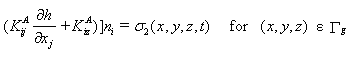
where g0 is a prescribed total gradient [LL-1] at the ΓG gradient-type boundary segments, and ni are the components of the outward unit vector normal to ΓG. This equation is commonly used to specify a unit vertical hydraulic gradient simulating free drainage from the bottom of a soil profile when the water table is situated far below the domain of interest. The condition is consistent with unit gradient conditions often observed in field studies of water flow, especially during redistribution (Sisson, 1987; McCord, 1991). Another possible application of this boundary condition is along the lateral sides of a hillslope, with the specified gradient being equal to the slope of the soil surface or some impermeable subsurface layer. Neither the flux nor the pressure head is then known a priori along the gradient boundary, but must be calculated from the (presumably numerical) solution.

System-Dependent Boundary Conditions

In many applications neither the flux across nor the pressure head or gradient along a boundary is known a priory, but follows from interactions between the vadose zone and its surroundings (e.g., the atmosphere or deeper subsurface). The boundary representing the soil air interface, which is exposed to atmospheric conditions, is one example of the system dependent boundary. The potential fluid flux across this interface is controlled exclusively by external conditions (precipitation, evaporation). However, the actual flux depends also on the (transient) moisture conditions in the soil. Soil surface boundary conditions may change from prescribed flux to prescribed head type conditions (and vice-versa). This occurs, for example, when the precipitation rate exceeds the infiltration capacity of the soil, resulting in either surface runoff or accumulation of excess water on top of the soil surface, depending upon the soil conditions. The infiltration rate in that case is not controlled any more by the precipitation rate, but instead by the infiltration capacity of the soil. A system-dependent boundary condition also occurs when the potential evaporation rate as calculated from meteorological conditions (the evaporative demand of the atmosphere), exceeds the capability of the soil to deliver enough water toward the soil surface. In this case the potential evaporation rate can be significantly reduced to an actual evaporation rate that is again controlled by the soil.

Atmospheric Boundary Condition:

System-dependent atmospheric boundary conditions can be implemented mathematically using an approach of Neuman et al. (1974) which limits the absolute value of the flux such that the following two conditions are satisfied:

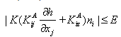
and

where E is the maximum potential rate of infiltration or evaporation under the current atmospheric conditions [LT-1], h is the pressure head at the soil surface [L], and hA and hS are, respectively, minimum and maximum pressure heads allowed under the prevailing soil conditions [L]. The value for hA is determined from the equilibrium conditions between soil water and atmospheric water vapor, whereas hS is usually set equal to zero (which would initiate instantaneous surface runoff) or results from the accumulation of excess water in the surface ponding layer, in which case its value must be calculated from the difference between the infiltration and precipitation (or irrigation) rates. When one of the limits is reached, a prescribed head boundary condition will be used to calculate the actual surface flux. Methods for calculating E and hA on the basis of atmospheric data have been discussed by Feddes et al. (1974).

Potential Evapotranspiration:

HYDRUS requires user to enter values of potential transpiration and potential evaporation for the atmospheric boundary conditions. HYDRUS then calculates the actual values of transpiration and evaporation based on the availability of water in the soil profile. The common problem is that users usually know the value of the potential evapotranpiration (calculated for example with the Penman-Monteith combination equation, e.g., FAO, etc.) and not directly its structural parts. Since HYDRUS does not have a crop growing module (does not calculate crop growth, various growth stages, leaf area index, etc) and concentrate only on movement of water and solute in the soil profile, it can not do this subdivision (into potential evaporation and potential transpiration) itself. The subdivision is different for each crop and is relatively complex. FAO and several other publications suggest using "Crop coefficient" which can be used to do this subdivision (into potential evaporation and potential transpiration). One can also use the Leaf Area Index (LAI) or Surface Fraction covered by plants to do this subdivision.

An example application of the atmospheric boundary condition for infiltration from a rainfall event is demonstrated in Figure below, which shows infiltration during and following rainfall at a large but constant intensity (50 cm/d) and of short duration (0.1 d) into a loamy soil. Calculations were carried out using HYDRUS-1D (Šimùnek et al., 2005) assuming that water can either pond at the soil surface or is immediately removed by surface runoff. Plots of both the pressure head and the infiltration rate show that surface ponding occurred after 0.0162 d. After this time the infiltration rate decreases continuously as time proceeds, with the reduction being smaller for the case with surface water build-up since the water level exerts a hydrostatic pressure at the soil surface. Infiltration ceased at the end of the infiltration event for the case that considered surface runoff. However, when water was allowed to accumulate on top of the soil surface, a 1.48-cm thick water layer developed at the end of the precipitation event, which subsequently served as a source for further infiltration until 0.156 d when all water had infiltrated. This simple application clearly demonstrates that neither the pressure head nor the water content could be specified at the boundary a priori, and that the actual flux depended on the interaction between the applied flux and the degree of saturation of the soil system.

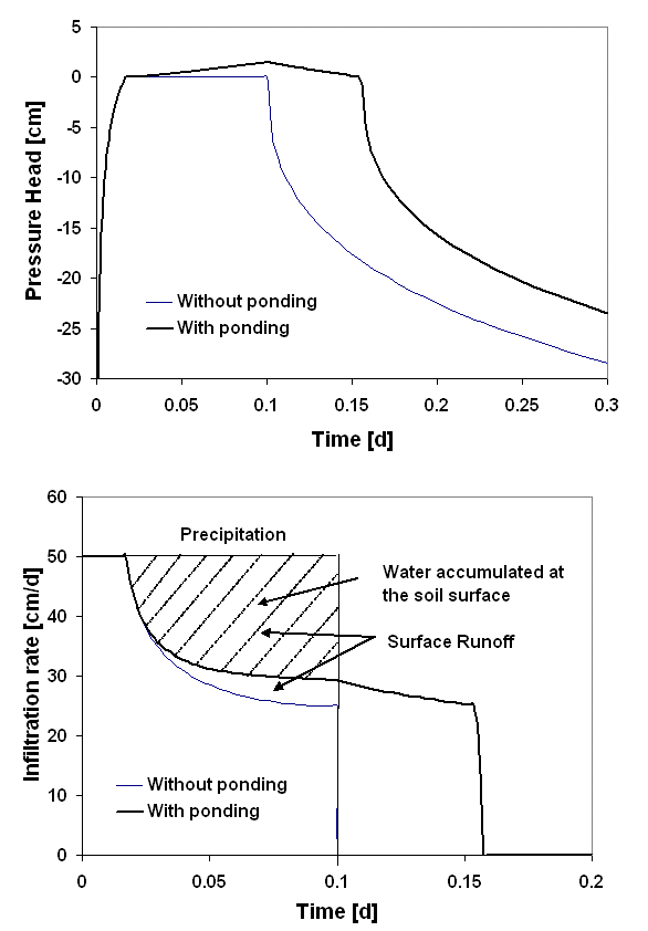
Infiltration from a high-intensity rain rainfall event in a loamy soil with and without surface ponding.

Overland flow:

HYDRUS does not directly calculate overland flow or the accumulation of water at the soil surface. HYDRUS assumes that all water in excess of the infiltration capacity is immediately lost to surface runoff. As the overland flow is in general much faster than the subsurface flow, this assumption is appropriate for a majority of applications.

Only in HYDRUS-1D we have an option that water can accumulate at the soil surface and possibly infiltrate later. Optionally, one can start with a certain depth of water standing at the soil surface and allow this water to infiltrate.

Seepage Face:

Another example of a system-dependent boundary condition is a seepage face through which water leaves the saturated part of the flow domain. The boundary condition in this case can be formulated mathematically as follows:

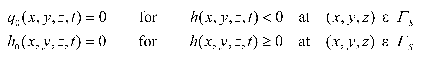
where ΓS are seepage face boundary segments. This boundary condition states that there is no flux across the boundary as long as the boundary is unsaturated, and that the pressure head is fixed to the zero value once saturation is reached. The flux across the boundary is then calculated from the flow field by solving the governing flow equations. This boundary condition can be used at the bottom of certain types of (finite) lysimeters, or along tile drains or the outflow part of dikes or riverbanks (Figure below). In the latter case the length of the seepage face is generally not known a priori and needs to be calculated.

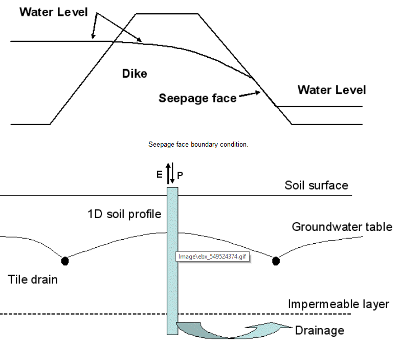
Equivalent tile drain boundary condition in one-dimensional flow formulation.

Tile Drain:

A special system-dependent boundary condition is sometimes implemented in one-dimensional numerical models (e.g., van Dam et al., 1997; Šimùnek et al., 2005) to account for flow to horizontal subsurface tile drains (Figure above). An equivalent drainage flux from the bottom of the simulated soil profile is then calculated using an appropriate analytical solutions for the tile drainage system (e.g., Houghoudt, 1940; Ernst, 1962; van Hoorn, 1997). The drainage equations involved generally hold for steady-state flow into the drain and depend upon the geometry of the system (e.g., depth of tile drain, depth to impermeable layer, location of water table midway between two drains, and possibly information about soil layering).

Deep Drainage:

Still other system-dependent boundary conditions can be formulated. One example is the use of a functional relationship between the position of the water table and drainage from (or infiltration into) the bottom boundary of the soil profile to account for regional flow effects (Hopmans and Stricker, 1989). Another example occurs when the water level in a furrow or a stream decreases, which may lead to a change in the applicable boundary condition from a specified head to a seepage face (with water then possibly flowing back from the soil profile to stream), with part of the seepage face exposed to atmospheric conditions. Unfortunately, few if any numerical models presently consider such dynamic changes between different types of surface boundary conditions.

Notes:

Note that Free Drainage and Deep Drainage boundary conditions can not be specified simultaneously in one project. Similarly, when the Gradient Boundary Condition is selected, the Time-Variable Flux 4 BC can not be applied in the same project.

See also the "How to Edit Boundary Conditions" topic.

See Boundary Conditions Options, Special Boundary Conditions, and Triggered Irrigation for additional information on boundary conditions.

Back to HYDRUS Step by Step.