In general, the hydraulic conductivity, K, can be different in different directions (e.g., horizontal and vertical direction). This phenomenon is called Anisotropy and is described by the Anisotropy Tensor. The Anisotropy Tensor in two-dimensional problems has dimensions of 2*2, and in three-dimensional problems 3*3.
Since the hydraulic anisotropy tensor, KA, is assumed to be symmetric, it is possible to define at any point in the flow domain a local coordinate system for which the tensor KA is diagonal (i.e., having zeros everywhere except on the diagonal). The diagonal entries K1A and K2A of KA are referred to as the principal components of KA.
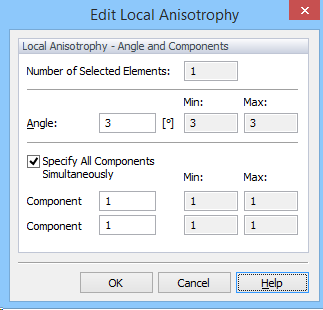
The local principal directions may be oriented differently from element to element. For this purpose, the local coordinate axes are subjected to a rotation such that they coincide with the principal directions of the tensor KA. The principal components K1A and K2A, together with the angle ω between the principal direction of K1A and the x-axis of the global coordinate system, are specified for each element.
Angle w between the principal direction of K1A and the x-axis of the global coordinate system |
|
The first principal component, K1A , of the dimensionless conductivity tensor KA |
|
The second principal component, K2A , of the dimensionless conductivity tensor KA |
|
Index representing the anisotropy tensor in three-dimensional applications |
The following commands are available in the Domain Properties part of the Edit Menu to define spatial distribution of Local Anisotropy:
See also the "How to Edit Domain Properties" topic.